This post describes how to setup a Python development environment suitable for machine learning on a Windows based system.

Let’s get started!

Table of Contents

• First: Install Python:
• Second: Install IPython and Jupyter Notebook:
  • Testing IPython (i.e. Command Line Execution)
  • Testing Jupyter Notebook (i.e. Notebook Execution)
  • Helpful Links and More Documentation on IPython and the Jupyter Notebook
• Third: Install Python Libraries:
  • StatsModels Library Install Issues
  • Python Library Details
• Fourth: Testing Jupyter Notebook
• Appendix A: Image Libraries
  • openCV
    • Install example:
    • Usage example:
  • Supporting HDF5 with h5py
    • Usage example:
      • Create and Write HDF5 Archive to Disk
      • Open and Read from HDF5 archive
• Appendix B: Other Helpful Items
  • Jupyter notebook extensions

First: Install Python:

Download the latest Python version and install it:

1. Browse to https://www.python.org/downloads/windows/
2. Click the Latest Python 3 Release - Python 3.6.4 hyperlink
3. Click the Windows x86-64 executable installer hyperlink
4. Browse to your download folder and double-click the python-3.6.4-amd64.exe file
5. Follow the prompts of the installer

(Don’t forget to allow the installer to add Python to your %PATH% environment variable…)

Second: Install IPython and Jupyter Notebook:

This part is pretty simple. We make a call to good ‘ol pip now that Python is installed:

1. Open a Windows PowerShell terminal
2. Execute the following command in the PowerShell terminal:

   pip install ipython jupyter
   

Next we’ll test out the IPython and Jupyter install to ensure we can 1) execute Python from the command line, and 2) execute Python from a Jupyter Notebook.

Testing IPython (i.e. Command Line Execution)

To confirm IPython was properly installed on your system:

1. Open a Windows PowerShell terminal
2. Execute the following command in the PowerShell terminal:

   ipython
   

You should see output similar to the following:

Python 3.6.4 (v3.6.4:d48eceb, Dec 19 2017, 06:54:40) [MSC v.1900 64 bit (AMD64)]
Type 'copyright', 'credits' or 'license' for more information
IPython 6.2.1 -- An enhanced Interactive Python. Type '?' for help.

In [1]:

Let’s try out a few commands:

In [1]:  print('Hello IPython')
Hello IPython

In [2]: 21 * 2
Out[2]: 42

In [3]: def say_hello(name):
   ...: 	print('Hello {name}'.format(name=name))

In [4]: say_hello("Python")
Hello Python

If everything appears the same in your console as the output above you should be set. :)

Helpful Links and More Documentation on IPython and the Jupyter Notebook

If you want to learn more about IPython and Jupyter Notebooks:

• Jupyter Notebook documentation
• iPython Tutorial

Third: Install Python Libraries:

We could worry about which libraries we should install to support our machine learning endeavors. Thankfully don’t have to; however, because there are two “stacks” already put together that contain most everything we’re likely to need. You can read about them at the following URLs:

• https://pydata.org/downloads.html
• https://www.scipy.org/stackspec.html

After reviewing the previous two stacks we’ll install the following libraries from them:

• NumPy
• SciPy
• Matplotlib
• Seaborn
• Pandas
• StatsModels
• Scikit-Learn

Obviously you can add or subtract as you see fit for your needs. :)

To install the libraries we’ve selected:

1. Open a Windows PowerShell terminal
2. Execute the following command in the PowerShell terminal:

   pip install numpy scipy matplotlib seaborn pandas statsmodels sklearn
   

StatsModels Library Install Issues

When I attempted to install the StatsModels library on my system I received the following error:

No module named 'numpy.distutils._msvccompiler' in numpy.distutils; trying from distutils
building 'statsmodels.tsa.kalmanf.kalman_loglike' extension
error: Microsoft Visual C++ 14.0 is required. Get it with "Microsoft Visual C++ Build Tools": http://landinghub.visualstudio.com/visual-cpp-build-tools

To resolve the issue I took the following steps:

1. Browse to http://landinghub.visualstudio.com/visual-cpp-build-tools
2. Download Visual C++ 2015 Build Tools
3. Execute the downloaded visualcppbuildtools_full.exe file
4. The installer will run, and once it does select a Custom installation and then click Next

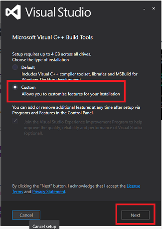
1. On the next screen that appears select Windows 8.1 SDK and then click Next

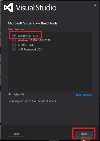
From here the installer will download the required files to complete the install. Please note this can take a while….

Once the installer completes restart the Windows PowerShell terminal, and execute the pip install command again:

pip install numpy scipy matplotlib seaborn pandas statsmodels sklearn

And we have success!

Installing collected packages: statsmodels
  Running setup.py install for statsmodels ... done
Successfully installed statsmodels-0.8.0

Python Library Details

Below is a summary for each library we’ve chosen along with a usage example:

• NumPy
  • URL: http://www.numpy.org/
  • Description: NumPy is the fundamental package for scientific computing with Python. It contains among other things: A powerful N-dimensional array object; sophisticated (broadcasting) functions; tools for integrating C/C++ and Fortran code; and useful linear algebra, Fourier transform, and random number capabilities. Besides its obvious scientific uses, NumPy can also be used as an efficient multi-dimensional container of generic data. Arbitrary data-types can be defined. This allows NumPy to seamlessly and speedily integrate with a wide variety of databases.
  • Usage example:

In [1]: import numpy as np

In [2]: a = np.arange(15).reshape(3, 5)
   ...: a
Out[2]:
array([[ 0,  1,  2,  3,  4],
       [ 5,  6,  7,  8,  9],
       [10, 11, 12, 13, 14]])

In [3]: a.shape
Out[3]: (3, 5)

• SciPy
  • URL: https://www.scipy.org/
  • Description: SciPy stands for Scientific Python. SciPy is a collection of mathematical algorithms and convenience functions built on the Numpy extension of Python. It adds significant power to the interactive Python session by providing the user with high-level commands and classes for manipulating and visualizing data. With SciPy an interactive Python session becomes a data-processing and system-prototyping environment rivaling systems such as MATLAB, IDL, Octave, R-Lab, and SciLab.
  • Usage example:

from scipy.interpolate import interp1d

x = np.linspace(0, 10, num=11, endpoint=True)
y = np.cos(-x**2/9.0)
f = interp1d(x, y)
f2 = interp1d(x, y, kind='cubic')

xnew = np.linspace(0, 10, num=41, endpoint=True)
import matplotlib.pyplot as plt
plt.plot(x, y, 'o', xnew, f(xnew), '-', xnew, f2(xnew), '--')
plt.legend(['data', 'linear', 'cubic'], loc='best')
plt.show()

• Matplotlib
  • URL: https://matplotlib.org/
  • Description: Matplotlib is a Python 2D plotting library which produces publication quality figures in a variety of hard copy formats and interactive environments across platforms. Matplotlib can be used in Python scripts, the Python and IPython shell, the jupyter notebook, web application servers, and four graphical user interface toolkits. You can generate plots, histograms, power spectra, bar charts, error charts, scatter plots, etc., with just a few lines of code
  • Usage example:

import numpy as np
import matplotlib
import matplotlib.pyplot as plt

# Fixing random state for reproducibility
np.random.seed(19680801)


matplotlib.rcParams['axes.unicode_minus'] = False
fig, ax = plt.subplots()
ax.plot(10*np.random.randn(100), 10*np.random.randn(100), 'o')
ax.set_title('Using hyphen instead of Unicode minus')
plt.show()

• Seaborn
  • URL: https://seaborn.pydata.org/
  • Description: Seaborn is a library for making attractive and informative statistical graphics in Python. It is built on top of matplotlib and tightly integrated with the PyData stack, including support for numpy and pandas data structures and statistical routines from scipy and statsmodels. Seaborn aims to make visualization a central part of exploring and understanding data. The plotting functions operate on data frames and arrays containing a whole dataset and internally perform the necessary aggregation and statistical model-fitting to produce informative plots. If matplotlib “tries to make easy things easy and hard things possible,” seaborn tries to make a well-defined set of hard things easy too.
  • Usage example:

import matplotlib.pyplot as plt
import seaborn as sns
sns.set(style="darkgrid", color_codes=True)

tips = sns.load_dataset("tips")
g = sns.jointplot("total_bill", "tip", data=tips, kind="reg",
    xlim=(0, 60), ylim=(0, 12), color="r", size=7)

plt.show()

• Pandas
  • URL: https://pandas.pydata.org/
  • Description: Pandas is utilized for data manipulation and analysis. In particular, it offers data structures and operations for manipulating numerical tables and time series.
  • Usage example:

import pandas as pd
import numpy as np
import matplotlib.pyplot as plt

dates = pd.date_range('20130101', periods=6)
df = pd.DataFrame(np.random.randn(6,4), index=dates, columns=list('ABCD'))
df

df.head()
df[df > 0]
df.apply(np.cumsum)

• StatsModels
  • URL: http://www.statsmodels.org/stable/index.html
  • Description: Statsmodels is a Python module that allows users to explore data, estimate statistical models, and perform statistical tests. An extensive list of descriptive statistics, statistical tests, plotting functions, and result statistics are available for different types of data and each estimator.
  • Usage example:

import numpy as np
import statsmodels.api as sm
import statsmodels.formula.api as smf

dat = sm.datasets.get_rdataset("Guerry", "HistData").data
results = smf.ols('Lottery ~ Literacy + np.log(Pop1831)', data=dat).fit()

print(results.summary())

• Scikit-Learn
  • URL: http://scikit-learn.org/stable/
  • Description: Scikit-learn (formerly scikits.learn) is a free software machine learning library for the Python programming language. It features various classification, regression and clustering algorithms including support vector machines, random forests, gradient boosting, k-means and DBSCAN, and is designed to interoperate with the Python numerical and scientific libraries NumPy and SciPy.
  • Usage example:

from sklearn import datasets
from sklearn.model_selection import cross_val_predict
from sklearn import linear_model
import matplotlib.pyplot as plt

lr = linear_model.LinearRegression()
boston = datasets.load_boston()
y = boston.target

# cross_val_predict returns an array of the same size as `y` where each entry
# is a prediction obtained by cross validation:
predicted = cross_val_predict(lr, boston.data, y, cv=10)

fig, ax = plt.subplots()
ax.scatter(y, predicted, edgecolors=(0, 0, 0))
ax.plot([y.min(), y.max()], [y.min(), y.max()], 'k--', lw=4)
ax.set_xlabel('Measured')
ax.set_ylabel('Predicted')
plt.show()

Fourth: Testing Jupyter Notebook

To confirm the Jupyter Notebook was properly installed on your system:

1. Open a Windows PowerShell terminal
2. Execute the following command in the PowerShell terminal:

   jupyter notebook
   

You should see output similar to the following:

> jupyter notebook
[I 10:19:29.384 NotebookApp] Serving notebooks from local directory: C:\Users\nzrasch\Documents\Development\python
[I 10:19:29.385 NotebookApp] 0 active kernels
[I 10:19:29.388 NotebookApp] The Jupyter Notebook is running at:
[I 10:19:29.391 NotebookApp] http://localhost:8888/?token=3b63e547f9f9803626caebba7129477e0e8e4b48fb5414c5
[I 10:19:29.393 NotebookApp] Use Control-C to stop this server and shut down all kernels (twice to skip confirmation).
[C 10:19:29.399 NotebookApp]

    Copy/paste this URL into your browser when you connect for the first time,
    to login with a token:
        http://localhost:8888/?token=3b63e547f9f9803626caebba7129477e0e8e4b48fb5414c5

(Note: On my system a browser window/tab automatically opens to the running notebook. If this doesn’t occur on your system paste the URL output found in the console when you started the notebook into your browser.)

Ex: http://localhost:8888/?token=3b63e547f9f9803626caebba7129477e0e8e4b48fb5414c5

Once you have the Jupyter Notebook running we can load some sample ipynb files and ensure everything looks good:

1. Browse to the directory where the envSetupTestOne.ipynb and envSetupTestTwo.ipynb files from this write-up were downloaded to. (Note: You can find them here on Github.)
2. Click the envSetupTestOne.ipynb and envSetupTestTwo.ipynb hyperlinks in the notebook file explorer area
3. The notebooks should execute in new tabs when you click them
4. For each notebook do the following:
5. Click Kernel -> Restart and Clear Output from the menu at the top of the notebook page
6. Click Cell -> Run All from the menu at the top of the notebook page
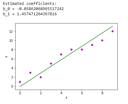
7. Confirm the text and graphical outputs at the bottom of the notebook pages contain the same items as in the screen shots below:

envSetupTestOne Output

envSetupTestTwo Output

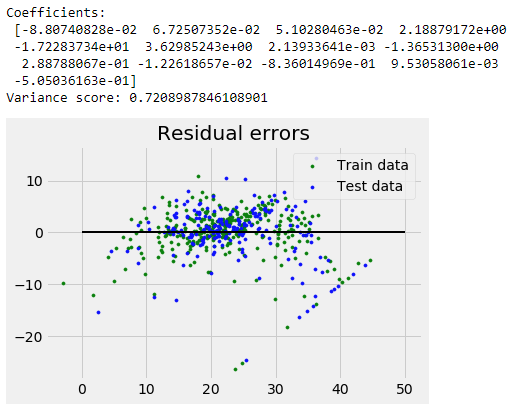
If the notebooks loaded and gave the same outputs as the screen shots above then you should be set. :)

Appendix A: Image Libraries

Below are an assortment of libraries I’ve found to be helpful when dealing with image processing.

openCV

• Browse to https://www.lfd.uci.edu/~gohlke/pythonlibs/#opencv

• Download the file that matches your python version.
  • Example: I have python v3.6, so I downloaded the file “opencv_python-3.4.0-cp36-cp36m-win_amd64.whl”
• Install it:
  1. Open a Windows PowerShell terminal
  2. Execute the following command in the PowerShell terminal:

     pip install <DOWNLOAD_PATH><filename>
     

Install example:

> pip install .\Downloads\opencv_python-3.4.0-cp36-cp36m-win_amd64.whl
Processing c:\users\nathan\downloads\opencv_python-3.4.0-cp36-cp36m-win_amd64.whl
Installing collected packages: opencv-python
Successfully installed opencv-python-3.4.0

You can find a quick tutorial and further documentation here.

Usage example:

# Display some number of images from a given directory
def displayImages(numberToShow, imagePath):
    # Container for the images we want to show in a grid
    images = []
    # Define what kind of images we want to iterate over
    imageFilter = os.path.join(imagePath, '**', '*.jpg')

    # Display the N number of images found in the given image director
    for filename in glob.iglob(imageFilter, recursive=True):
        image = cv2.imread(filename, cv2.IMREAD_COLOR)
        image = cv2.cvtColor(image, cv2.COLOR_BGR2RGB)
        images.append(image)
        if len(images) == numberToShow:
            break

    # Show the images we've collected
    grid_display(images, [], 5, (10,10))

    return

Supporting HDF5 with h5py

1. Open a Windows PowerShell terminal
2. Execute the following command in the PowerShell terminal:

   pip install h5py
   

Usage example:

Create and Write HDF5 Archive to Disk

# Write the train and test labels and images to a HDF5 container
def createArchive(outputFile, trainLabels, testLabels, trainImages, testImages, features = 12288):
    # Create the HDF5 container and add the sample data we've created
    with h5py.File(outputFile, "w") as archive:
        archive.create_dataset("trainLabels", data=trainLabels)
        archive.create_dataset("testLabels", data=testLabels)
        archive.create_dataset("trainImages", data=flattenImages(features, trainImages))
        archive.create_dataset("testImages", data=flattenImages(features, testImages))
        archive.close()

    # Check the size on disk
    sizeOnDisk = round(os.path.getsize(outputFile) / 1024, 1)
    print(str(outputFile) + " file size (kb): " + str(sizeOnDisk))

    return archive

Open and Read from HDF5 archive

# Quick and dirty test to ensure the HDF5 archive file was created correctly
def validateArchive(archiveFile):
    # Open and read the HDF5 container
    with h5py.File(archiveFile, "r") as archive:
        print("HDF5 container keys: " + str(list(archive.keys())) + "\n")

        # Pull the train labels from the HDF5 container
        cData = archive['trainLabels']
        print("Train labels:")
        print(list(cData))
        print("\n")

        # Pull the train data from the HDF5 container
        cData = archive['trainImages']
        # Pull first image and examine it
        item = cData[:, 0]
        print("First HDF5 container dataSet item shape: " + str(item.shape))
        print("First 10 dataSet item one values:")
        print(item[1:10])
        print("\n")

        # View the image
        image = item.reshape((64, 64, 3))*255
        cv2.imwrite('archiveTest.jpg', image)
        image = cv2.imread('archiveTest.jpg', cv2.IMREAD_COLOR)
        image = cv2.cvtColor(image, cv2.COLOR_BGR2RGB)
        plt.imshow(image)

        # Close the HDF5 container
        archive.close()

    return

Appendix B: Other Helpful Items

Jupyter notebook extensions

This is a great collection of added functionality for Jupyter Notebooks. For example, it adds support for spell checking, code folding, etc.

You can find the github repository for it here: https://github.com/ipython-contrib/jupyter_contrib_nbextensions

• Install it:
  1. Open a Windows PowerShell terminal
  2. Execute the following command in the PowerShell terminal:

     pip install https://github.com/ipython-contrib/jupyter_contrib_nbextensions/tarball/master
     jupyter contrib nbextension install --user
     

Next, I highly recommend you also install the the jupyter_nbextensions_configurator server extension which is installed as a dependency of nbextensions, and can be used to enable and disable the individual nbextensions, as well as configure their options.

• Install it:
  1. Open a Windows PowerShell terminal
  2. Execute the following command in the PowerShell terminal:

     pip install jupyter_nbextensions_configurator
     jupyter nbextensions_configurator enable --user
     

Here is a screen shot of what the Jupyter nbextensions configurator server UI looks like once installed. The new nbextension tab is circled in red, as well as the option to enable spell checking:

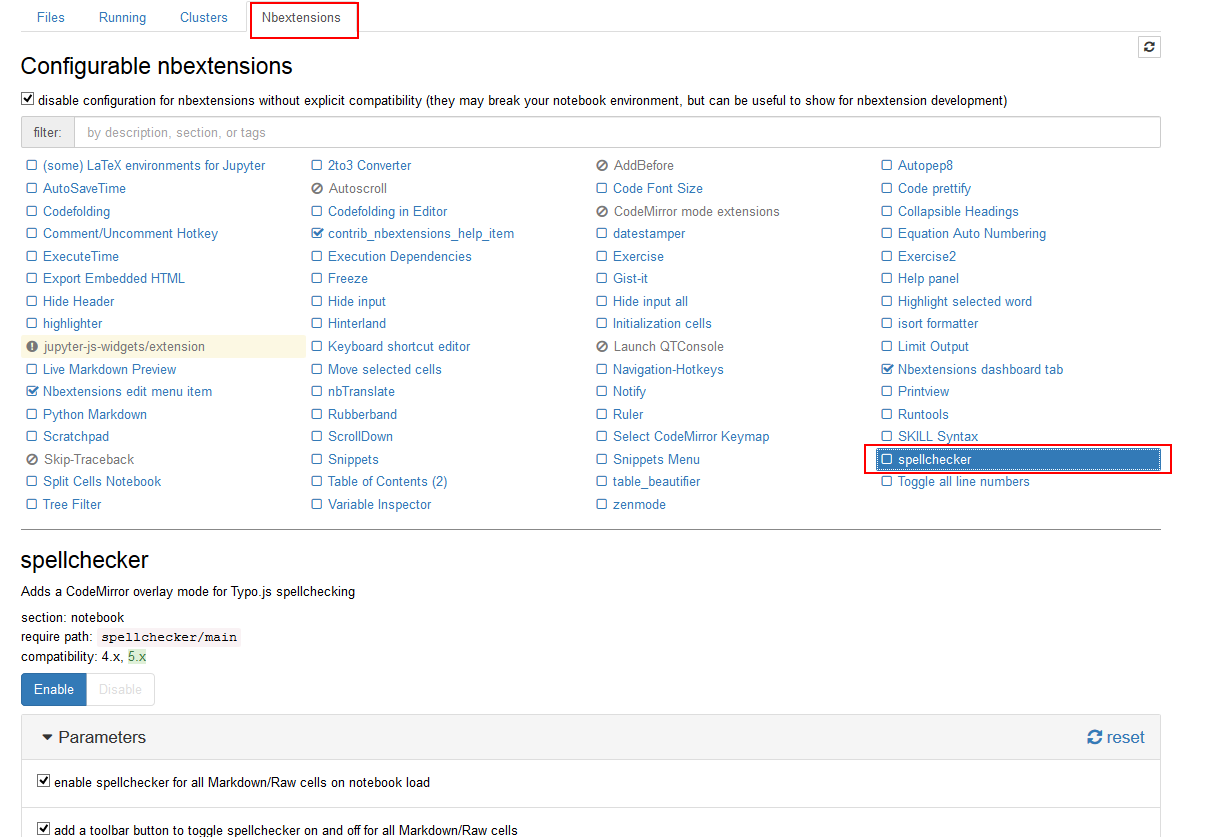
You can easily select the items you want to enable as well as read more about what each extension does. Very handy!